The article highlights key ideas used in popular and successful versions of BERT. An understanding of BERT Transformer is required to fully grasp the article. Please refrain from directly copying content from the post. In case you want to use an excerpt or any original image, mention the link to the post.

Last weekend I went on a BERT-paper reading spree. I have been familiar with BERT for quite a while now, but the moment you read a BERT paper, probably there’s a researcher in a lab who’s burning GPUs on some new BERT version.

It’s freaking hard to keep track of all BERTs - BERT, Distil BERT, ALBERT, RoBERTa, TinyBERT, Longformer, etc. At first, I thought why to bother reading about every BERT version. Let’s wait and see who wins.

However, here’s what I realized -

Don’t fish for the winner. Fish for the ideas.

Instead of focusing on which BERT performs well, I started focusing on the ideas each version of BERT uses.

Ideas in Data Science are transferrable from one domain to another. SOTA performance is rarely reproducible on your specific problem.

This post is more like a handy reference than a tutorial or explanation. I mainly focus on the ideas that makes each of these models different.

Concept of Query, Key and Values in self-attention

When I first read about query, key and values in the paper Attention is all you need, I was confused. I could not relate the terms to the matrix operations happening in the self-attention layer. Soon I realized that it is very similar to Python dictionaries. In fact, it is nothing new at all!

Consider a dictionary my_dict with keys and values. When you make a query like my_dict[some_key], Python does an exact match of the query with the keys present in the dictionary. If the key is present, it returns a value, else it throws an error. Let’s call it hard-match. Think of it like you have M keys and a valid query will generate a one-hot vector of size M with one of the positions as 1 (where some_key is present) and the rest as 0.

BERT does something similar, except it is a soft-match. The query is a distributed vector representation. The keys are distributed keys. A matrix multiplication and then a softmax operation generates a vector of size M. Only this time the probability mass is distributed across keys (or words) instead of being one-hot.

Who’s faster - self-attention or RNN?

To take full advantage of parallel computing, we need as few sequential steps as possible. In RNNs, you need to finish computing the previous time-steps to start with a new one. Since RNNs are sequential by nature, parallelization is restricted.

The paper Attention is all you need provides a big-O time complexity analysis of various architectures. There are two components here - time complexity per layer and number of sequential operation.

Self-Attention -

Complexity per layer - O(d*n^2). d is the embedding dimension. n^2 because it computes attention weights for each word with respect to every other word. O(n) operations for each word and therefore O(n^2) for all the words.
Number of sequential steps - O(1). All n operations happen in a single time-step. Note that although all the N tokens are processed, none of them are sequential like a standard RNN.

RNN -

Complexity per layer - O(n*d^2). Matrix multiplication of the previous step’s hidden states with the weight matrix takes d^2 operations. For n-steps to be processed, O(n*d^2) operations are needed.
Number of sequential steps - O(n). All n operations happen in n time-step. Note that all the n tokens are processed sequentially.

So who is faster?

Now, n ranges from 1 to a few hundreds in monst cases. d ranges from hundreds to thousands (512-1024)

For n<d, which is a common cause, self-attention is faster. In addition, due to the minimum number of sequential steps it requires, it can be parallelized very easily.

Breaking the hidden-dimension barrier

Most NLP models deal with the problem of large vocabulary size. Apart from covering all possible words, another issue is that size of the model increases very quickly. In transformers, embedding matrix is of size (vocab_size, hidden_dimension). For large vocabularies like 50,000, doubling hidden dimension size from 512 to 1024 introduces 25.6 million parameters.

ALBERT, a lite version of BERT proposes a matrix factorization approach to solve this problem. If we decompose the embedding matrix into 2 matrices of size (vocab_size, some_dim) and (some_dim, hidden_dimension), we can grow the hidden_dimension without worrying too much about the memory used.

Is NSP too easy??

BERT uses a self-supervised loss called Next Sentence Prediction (NSP). The objective is to predict if, among a pair of sentences, the first sentence precedes the second one. Creating training data for this task is easy. Positive examples are built by picking consecutive sentence pair at random. Negative examples are built by picking ANY two sentences at random.

Authors of ALBERT argue that NSP is too easy. And there is a legitimate reason for that. If the model learns to predict the topic of sentences well, NSP is kinda solved. For negative examples, the pair would belong to different topics (since they are random). For positive examples, sentences would belong to the same topic (since they are consecutive).

ALBERT uses an arguably more difficult objective called Sentence Order Prediction (SOP). The model has to predict if two sentences are in the correct order. Positive examples are created similar to NSP. Negative examples are created by swapping a randomly sampled pair of consecutive sentences. Here, just knowing the topic won’t suffice. Model is forced to learn more fine-grained features.

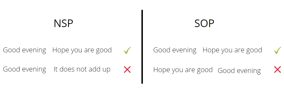
Original Image. Positive and negative examples in NSP and SOP.

Towards smaller BERTs

TinyBERT and DistilBERT have been quite popular as small but effective versions of BERT. They use Distillation to train a smaller version of BERT that learns from a bigger version of BERT. This is called a student-teacher framework.

While calculating the cross-entropy loss for student model’s prediction, the log probabilities of student network are multiplied with softmax probabilities of teacher network and then added, instead of using normal one-hot labels.

The idea of distillation is quite old though. It was proposed by Hinton in 2015.

Transformers beyond 512 tokens

As discussed earlier, self-attention scales quadratically with the sequence length. This limits BERT’s capability to process documents with more than 512 tokens. To process such documents there have been approaches to fragment to documents such that each fragment is shorter than 512 tokens. This loses crucial inter-fragment information and is sub-optimal.

Longformer uses a different way to approach attention. It uses a hybrid of local and global attention. In local attention, a word attends to a fixed number of neighbors. In global attention, a word attends to all the words in the sequence, just like in BERT. Local attention works in linear time. More specifically O(n*m) time, where m is the window size.

The idea behind the hybrid is to use local attention for MLM tasks and global attention for classification tasks where it is important for the [CLS] token to account for every word.

GAN - Like pre-training of transformers

ELECTRA uses a GAN-like (not GAN though) approach to pre-train a transformer. It jointly trains 2 networks - a generator and a discriminator. For an input sequence, random tokens are masked with a [MASK] token. This masked input is fed to the generator. The generator learns to predict these masked tokens via maximum-likelihood training. The generator predicted sentence (original non-masked tokens + masked token predictions by the generator) are then fed to the discriminator. The discriminator tried to predict which tokens are replaced and which are the original.

Unlike GANs, the masked predicted token is not considered fake. it is a valid real token. This is one key difference between how GANs are formulated vs how ELECTRA is formulated. Another difference is that the generator is not supplied with a noise vector as input, which happens in GANs

Conclusion

As a newbie, I used to focus on which model is the best for a task. With experience, I learned that not having a SOTA model is rarely the problem. Eventually, I started asking What works for my data and my business use-case?

In software applications, you usually pre-compute and save things to avoid computing things again and again. I think something similar applies to learning. You just try to know as many useful things as possible so that when a new problem comes up, you have a suite of possible solutions up your sleeve.

Hope the article was worth your time :)

BERT-ology at 100 kmph